Kaggle - Classification with Bank Churn
1. Projet
L’objectif de ce projet est de prédire si un client va continuer à utiliser les services de la banque ou s’il va clôturer son compte (churn)
2. Analyse des données
lecture du dataset
df = pd.read_csv(f'{os.path.dirname(__file__)}/kaggle/bank_churn_train_data.csv')
            ID  CustomerId  ... EstimatedSalary  Exited
0        37765    15794860  ...       161205.61       0
1       130453    15728005  ...       181419.29       0
2        77297    15686810  ...       100862.54       0
3        40858    15760244  ...        61164.45       1
4        19804    15810563  ...       103737.82       0
...        ...         ...  ...             ...     ...
143574   97639    15759915  ...       103349.74       0
143575   95939    15769974  ...       121299.14       0
143576  152315    15592028  ...        57569.89       0
143577  117952    15804009  ...        84496.78       0
143578   43567    15771409  ...       140937.98       1

[143579 rows x 14 columns]
df.head()
       ID  CustomerId     Surname  ...  IsActiveMember EstimatedSalary Exited
0   37765    15794860      Ch'eng  ...             1.0       161205.61      0
1  130453    15728005  Hargreaves  ...             1.0       181419.29      0
2   77297    15686810       Ts'ui  ...             1.0       100862.54      0
3   40858    15760244   Trevisano  ...             0.0        61164.45      1
4   19804    15810563      French  ...             1.0       103737.82      0

[5 rows x 14 columns]
df.describe()
                  ID    CustomerId  ...  EstimatedSalary         Exited
count  143579.000000  1.435790e+05  ...    143579.000000  143579.000000
mean    82521.171097  1.569202e+07  ...    112530.072465       0.212078
std     47650.353367  7.142049e+04  ...     50301.718378       0.408781
min         0.000000  1.556570e+07  ...        11.580000       0.000000
25%     41259.500000  1.563299e+07  ...     74580.800000       0.000000
50%     82485.000000  1.569018e+07  ...    117931.100000       0.000000
75%    123793.500000  1.575685e+07  ...    155149.685000       0.000000
max    165033.000000  1.581569e+07  ...    199992.480000       1.000000

[8 rows x 11 columns]
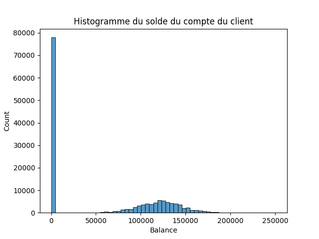
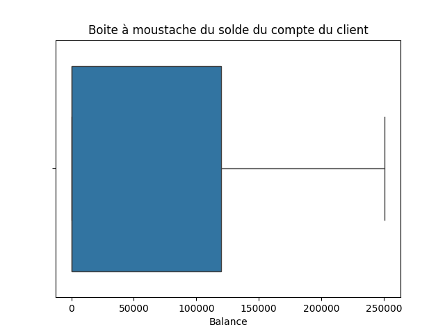
Variable continue : 'Balance
Balance : Le solde du compte du client
df['Balance'].describe()
count    143579.000000
mean      55533.640642
std       62822.616346
min           0.000000
25%           0.000000
50%           0.000000
75%      119948.090000
max      250898.090000
Name: Balance, dtype: float64
sns.histplot(data=df, x='Balance')
sns.boxplot(data=df, x='Balance')
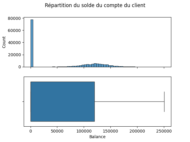
fig, ax = plt.subplots(2, 1, sharex=True)
plt.suptitle('Répartition du solde du compte du client')
sns.histplot(data=df, x='Balance', ax=ax[0])
sns.boxplot(data=df, x='Balance', ax=ax[1])
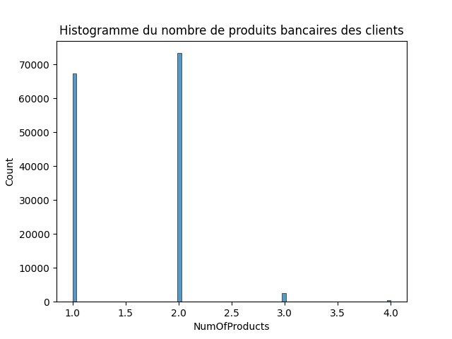
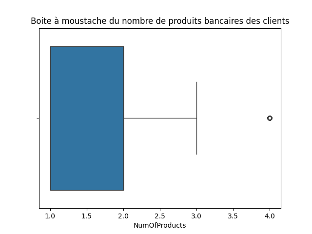
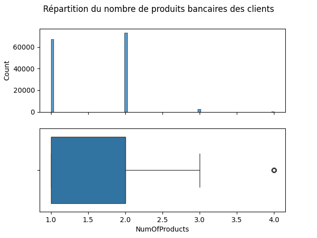
Variable continue : 'NumOfProducts
NumOfProducts : Le nombre de produits bancaires utilisés par le client (par exemple, compte d’épargne, carte de crédit)
df['NumOfProducts'].describe()
count    143579.000000
mean          1.553932
std           0.546754
min           1.000000
25%           1.000000
50%           2.000000
75%           2.000000
max           4.000000
Name: NumOfProducts, dtype: float64
sns.histplot(data=df, x='NumOfProducts')
sns.boxplot(data=df, x='NumOfProducts')
fig, ax = plt.subplots(2, 1, sharex=True)
plt.suptitle('Répartition du nombre de produits bancaires des clients')
sns.histplot(data=df, x='NumOfProducts', ax=ax[0])
sns.boxplot(data=df, x='NumOfProducts', ax=ax[1])
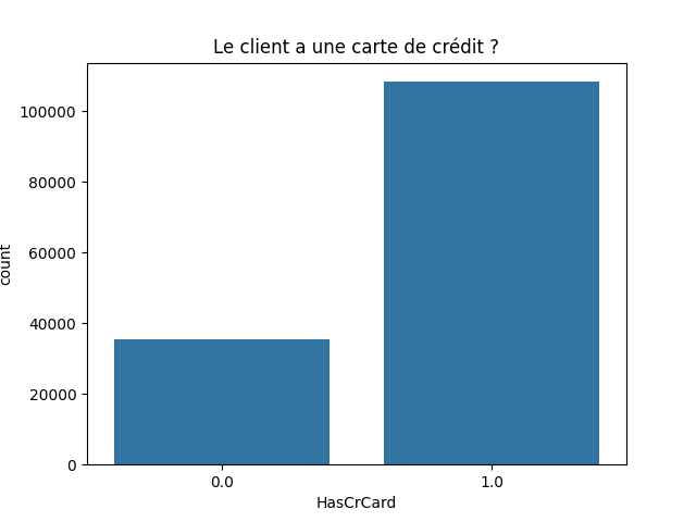
Variable discrète : 'HasCrCard
HasCrCard : Si le client possède une carte de crédit (1 = oui, 0 = non)
calcul des effectifs
df['HasCrCard'].value_counts(normalize=False, sort=True, ascending=False)
HasCrCard
1.0    108274
0.0     35305
Name: count, dtype: int64
distribution des effectifs
df['HasCrCard'].value_counts(normalize=False, sort=True, ascending=False)
HasCrCard
1.0    0.754107
0.0    0.245893
Name: proportion, dtype: float64
sns.scatterplot(data=df, x='HasCrdCart')
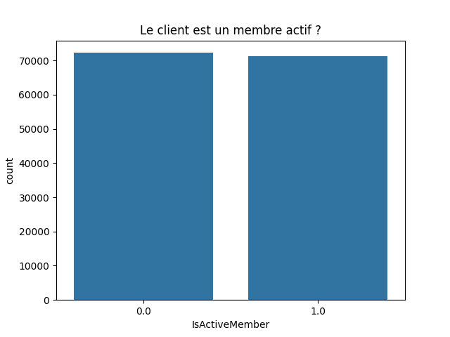
Variable discrète : 'IsActiveMember
IsActiveMember : Si le client est un membre actif (1 = oui, 0 = non)
calcul des effectifs
df['IsActiveMember'].value_counts(normalize=False, sort=True, ascending=False)
IsActiveMember
0.0    72249
1.0    71330
Name: count, dtype: int64
distribution des effectifs
df['IsActiveMember'].value_counts(normalize=False, sort=True, ascending=False)
IsActiveMember
0.0    0.5032
1.0    0.4968
Name: proportion, dtype: float64
sns.scatterplot(data=df, x='HasCrdCart')
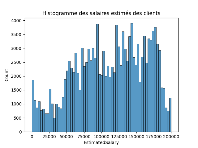
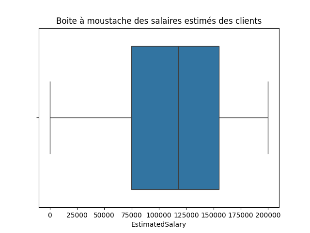
Variable continue : 'EstimatedSalary
EstimatedSalary : Le salaire estimé du client
df['EstimatedSalary'].describe()
count    143579.000000
mean     112530.072465
std       50301.718378
min          11.580000
25%       74580.800000
50%      117931.100000
75%      155149.685000
max      199992.480000
Name: EstimatedSalary, dtype: float64
sns.histplot(data=df, x='EstimatedSalary')
sns.boxplot(data=df, x='EstimatedSalary')
fig, ax = plt.subplots(2, 1, sharex=True)
plt.suptitle('Répartition des salaires estimés des clients')
sns.histplot(data=df, x='EstimatedSalary', ax=ax[0])
sns.boxplot(data=df, x='EstimatedSalary', ax=ax[1])

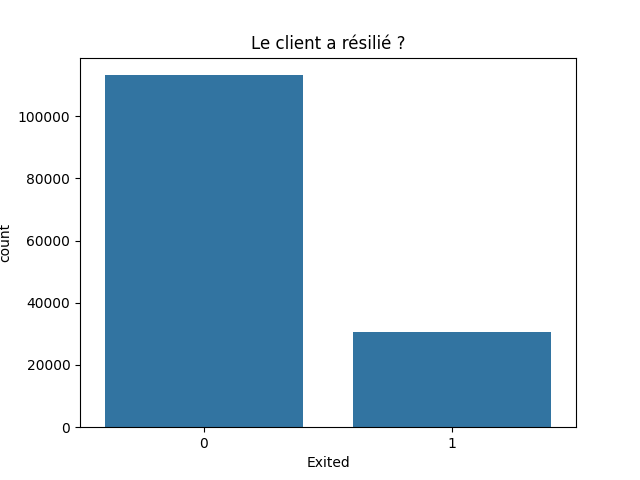
Variable discrète : 'Exited
(La target) Exited : Si le client a résilié (1 = oui, 0 = non)
calcul des effectifs
df['Exited'].value_counts(normalize=False, sort=True, ascending=False)
Exited
0    113129
1     30450
Name: count, dtype: int64
distribution des effectifs
df['Exited'].value_counts(normalize=False, sort=True, ascending=False)
Exited
0    0.787922
1    0.212078
Name: proportion, dtype: float64
sns.scatterplot(data=df, x='Exited')
3. Traitement des données
EstimatedSalary: Normalization MinMax
Modèle de Classification KNeighborsClassifier
4. Make predictions
lecture du dataset de test
df = pd.read_csv(f'{os.path.dirname(__file__)}/kaggle/bank_churn_test_data.csv')
           ID  CustomerId  ... EstimatedSalary  Salary_Normalized
0       67897    15585246  ...        91830.75           0.459140
1      163075    15604551  ...        90876.95           0.454370
2      134760    15729040  ...        47777.15           0.238851
3       68707    15792329  ...        82696.84           0.413466
4        3428    15617166  ...       151887.16           0.759450
...       ...         ...  ...             ...                ...
21450   24790    15697574  ...       175072.47           0.875388
21451  152608    15682708  ...       156680.71           0.783420
21452   28134    15614215  ...       173599.38           0.868022
21453  123871    15587573  ...       161479.19           0.807415
21454   98510    15598070  ...        62390.59           0.311925

[21455 rows x 14 columns]
Prédictions
df = pd.read_csv(f'{os.path.dirname(__file__)}/kaggle/bank_churn_test_data.csv')
scaler = MinMaxScaler()
df['Salary_Normalized'] = scaler.fit_transform(df[['EstimatedSalary']])
X_new = df[['HasCrCard', 'IsActiveMember', 'Salary_Normalized']]
predictions = model.predict(X_new)
[0 0 0 ... 0 1 0]
Submission
results = pd.DataFrame(
    {
        'ID': df['ID'],
        'Exited': predictions
    }
)
results = results.set_index('ID')
        Exited
ID
67897        0
163075       0
134760       0
68707        0
3428         0
...        ...
24790        0
152608       0
28134        0
123871       1
98510        0

[21455 rows x 1 columns]