Diamonds - Normalization
1. Analyse du dataset pour l'encodage
2. Analyse du dataset pour la normalisation
3. Normalization MinMax
4. Standartisation - Carat
5. Standartisation - Depth
6. MinMax - Price
2. Analyse du dataset pour la normalisation
3. Normalization MinMax
4. Standartisation - Carat
5. Standartisation - Depth
6. MinMax - Price
1. Analyse du dataset pour l'encodage
Analyse du Dataset
df = sns.load_dataset('diamonds')
df.head()
   carat      cut color clarity  depth  table  price     x     y     z
0   0.23    Ideal     E     SI2   61.5   55.0    326  3.95  3.98  2.43
1   0.21  Premium     E     SI1   59.8   61.0    326  3.89  3.84  2.31
2   0.23     Good     E     VS1   56.9   65.0    327  4.05  4.07  2.31
3   0.29  Premium     I     VS2   62.4   58.0    334  4.20  4.23  2.63
4   0.31     Good     J     SI2   63.3   58.0    335  4.34  4.35  2.75
2. Analyse du dataset pour la normalisation
df_numeric = df.select_dtypes(exclude='category')
df_numeric.describe(include='all', exclude = None)
              carat         depth  ...             y             z
count  53940.000000  53940.000000  ...  53940.000000  53940.000000
mean       0.797940     61.749405  ...      5.734526      3.538734
std        0.474011      1.432621  ...      1.142135      0.705699
min        0.200000     43.000000  ...      0.000000      0.000000
25%        0.400000     61.000000  ...      4.720000      2.910000
50%        0.700000     61.800000  ...      5.710000      3.530000
75%        1.040000     62.500000  ...      6.540000      4.040000
max        5.010000     79.000000  ...     58.900000     31.800000

[8 rows x 7 columns]
Les variables numériques sont 'carat', 'depth', 'table', 'price', 'x', 'y', 'z'
Variable 'carat'

fig,ax = plt.subplots(2, 1)
sns.histplot(data=df_numeric, x='carat', ax=ax[0])
sns.boxplot(data=df_numeric, x='carat', ax=ax[1])
plt.tight_layout()
Conclusion pour la variable 'carat'
Beaucoup de outliers et pas d'allure Gaussienne
Il faudra décomposer la variable 'carat' en plusieurs sous-variables...
Beaucoup de outliers et pas d'allure Gaussienne
Il faudra décomposer la variable 'carat' en plusieurs sous-variables...
Variable 'depth'

fig,ax = plt.subplots(2, 1)
sns.histplot(data=df_numeric, x='depth', ax=ax[0])
sns.boxplot(data=df_numeric, x='depth', ax=ax[1])
plt.tight_layout()
Conclusion pour la variable 'depth'
Beaucoup de outliers mais une allure Gaussienne
=> Normalisation par Standardisation
Beaucoup de outliers mais une allure Gaussienne
=> Normalisation par Standardisation
Variable 'table'

fig,ax = plt.subplots(2, 1)
sns.histplot(data=df_numeric, x='table', ax=ax[0])
sns.boxplot(data=df_numeric, x='table', ax=ax[1])
plt.tight_layout()
Conclusion pour la variable 'table'
Beaucoup de outliers mais une allure Gaussienne
=> Normalisation par Standardisation
Beaucoup de outliers mais une allure Gaussienne
=> Normalisation par Standardisation
Variable 'price'
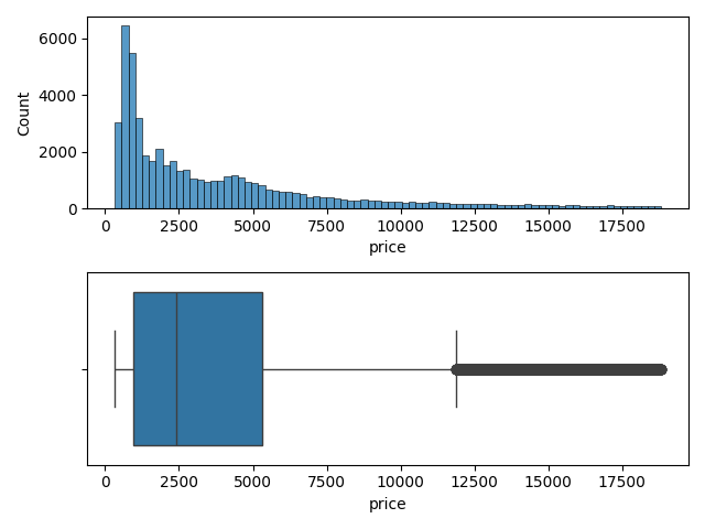
fig,ax = plt.subplots(2, 1)
sns.histplot(data=df_numeric, x='price', ax=ax[0])
sns.boxplot(data=df_numeric, x='price', ax=ax[1])
plt.tight_layout()
Conclusion pour la variable 'price'
Beaucoup de outliers et pas d'allure Gaussienne
=> Normalisation MinMax
Beaucoup de outliers et pas d'allure Gaussienne
=> Normalisation MinMax
Variable 'x'
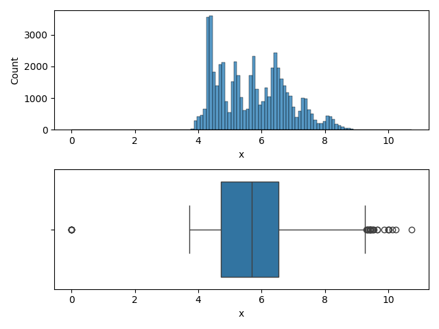
fig,ax = plt.subplots(2, 1)
sns.histplot(data=df_numeric, x='x', ax=ax[0])
sns.boxplot(data=df_numeric, x='x', ax=ax[1])
plt.tight_layout()
Conclusion pour la variable 'x'
Des outliers et une allure Gaussienne => Standardisation
Des outliers et une allure Gaussienne => Standardisation
Variable 'y'
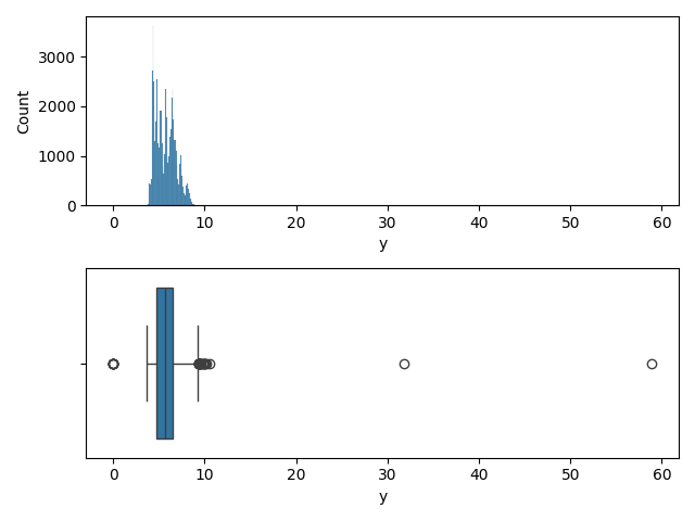
fig,ax = plt.subplots(2, 1)
sns.histplot(data=df_numeric, x='y', ax=ax[0])
sns.boxplot(data=df_numeric, x='y', ax=ax[1])
plt.tight_layout()
Conclusion pour la variable 'y'
Des outliers et une allure Gaussienne => Standardisation
Des outliers et une allure Gaussienne => Standardisation
Variable 'z'
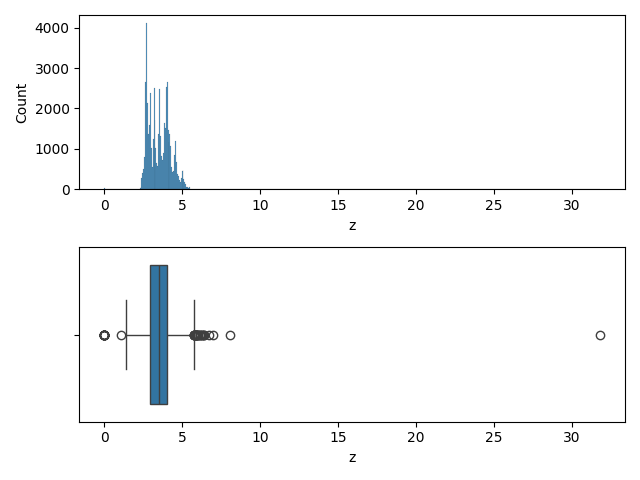
fig,ax = plt.subplots(2, 1)
sns.histplot(data=df_numeric, x='z', ax=ax[0])
sns.boxplot(data=df_numeric, x='z', ax=ax[1])
plt.tight_layout()
Conclusion pour la variable 'z'
Des outliers et une allure Gaussienne => Standardisation
Des outliers et une allure Gaussienne => Standardisation
3. Normalization MinMax
- convient pour la plupart des distributions
- à éviter pour les valeurs aberrantes
- à éviter pour les valeurs aberrantes
MinMaxScaler
from sklearn.preprocessing import MinMaxScaler

scaler = MinMaxScaler()
scaler.fit(df_numeric)
scaler.transform(df_numeric)
          carat     depth     table     price         x         y         z
0      0.006237  0.513889  0.230769  0.000000  0.367784  0.067572  0.076415
1      0.002079  0.466667  0.346154  0.000000  0.362197  0.065195  0.072642
2      0.006237  0.386111  0.423077  0.000054  0.377095  0.069100  0.072642
3      0.018711  0.538889  0.288462  0.000433  0.391061  0.071817  0.082704
4      0.022869  0.563889  0.288462  0.000487  0.404097  0.073854  0.086478
...         ...       ...       ...       ...       ...       ...       ...
53935  0.108108  0.494444  0.269231  0.131427  0.535382  0.097793  0.110063
53936  0.108108  0.558333  0.230769  0.131427  0.529795  0.097623  0.113522
53937  0.103950  0.550000  0.326923  0.131427  0.527002  0.096435  0.111950
53938  0.137214  0.500000  0.288462  0.131427  0.572626  0.103905  0.117610
53939  0.114345  0.533333  0.230769  0.131427  0.542831  0.099660  0.114465

[53940 rows x 7 columns]
MinMaxScaler
from sklearn.preprocessing import MinMaxScaler

scaler = MinMaxScaler()
scaler.fit(df_numeric)
df_minmax = pd.DataFrame(scaler.transform(df_numeric), columns=df_numeric.columns)
          carat     depth     table     price         x         y         z
0      0.006237  0.513889  0.230769  0.000000  0.367784  0.067572  0.076415
1      0.002079  0.466667  0.346154  0.000000  0.362197  0.065195  0.072642
2      0.006237  0.386111  0.423077  0.000054  0.377095  0.069100  0.072642
3      0.018711  0.538889  0.288462  0.000433  0.391061  0.071817  0.082704
4      0.022869  0.563889  0.288462  0.000487  0.404097  0.073854  0.086478
...         ...       ...       ...       ...       ...       ...       ...
53935  0.108108  0.494444  0.269231  0.131427  0.535382  0.097793  0.110063
53936  0.108108  0.558333  0.230769  0.131427  0.529795  0.097623  0.113522
53937  0.103950  0.550000  0.326923  0.131427  0.527002  0.096435  0.111950
53938  0.137214  0.500000  0.288462  0.131427  0.572626  0.103905  0.117610
53939  0.114345  0.533333  0.230769  0.131427  0.542831  0.099660  0.114465

[53940 rows x 7 columns]
df_minmax.describe()
              carat         depth  ...             y             z
count  53940.000000  53940.000000  ...  53940.000000  53940.000000
mean       0.124312      0.520817  ...      0.097360      0.111281
std        0.098547      0.039795  ...      0.019391      0.022192
min        0.000000      0.000000  ...      0.000000      0.000000
25%        0.041580      0.500000  ...      0.080136      0.091509
50%        0.103950      0.522222  ...      0.096944      0.111006
75%        0.174636      0.541667  ...      0.111036      0.127044
max        1.000000      1.000000  ...      1.000000      1.000000

[8 rows x 7 columns]
Comparatif df_numeric et df_minmax
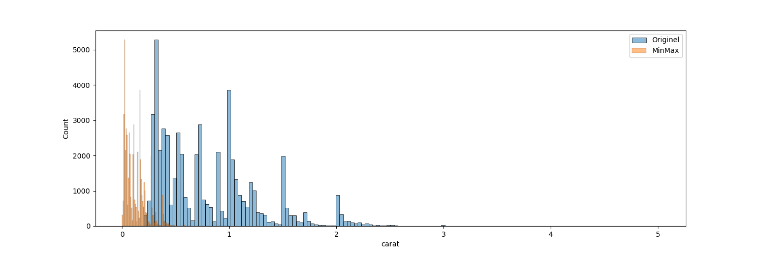
plt.figure(figsize=(15,5))
sns.histplot(data=df_numeric, x='carat', color='tab:blue', alpha=0.5)
sns.histplot(data=df_minmax, x='carat', color='tab:orange', alpha=0.5)
4. Standartisation - Carat
- Donne de bons résultats aux variables suivant une allure Gaussienne
StandardScaler
from sklearn.preprocessing import StandardScaler

scaler = StandardScaler()
scaler.fit(df_numeric)
df_standard = pd.dataFrame(scaler.transform(df_numeric), columns=df_numeric.columns)
          carat     depth     table     price         x         y         z
0      0.006237  0.513889  0.230769  0.000000  0.367784  0.067572  0.076415
1      0.002079  0.466667  0.346154  0.000000  0.362197  0.065195  0.072642
2      0.006237  0.386111  0.423077  0.000054  0.377095  0.069100  0.072642
3      0.018711  0.538889  0.288462  0.000433  0.391061  0.071817  0.082704
4      0.022869  0.563889  0.288462  0.000487  0.404097  0.073854  0.086478
...         ...       ...       ...       ...       ...       ...       ...
53935  0.108108  0.494444  0.269231  0.131427  0.535382  0.097793  0.110063
53936  0.108108  0.558333  0.230769  0.131427  0.529795  0.097623  0.113522
53937  0.103950  0.550000  0.326923  0.131427  0.527002  0.096435  0.111950
53938  0.137214  0.500000  0.288462  0.131427  0.572626  0.103905  0.117610
53939  0.114345  0.533333  0.230769  0.131427  0.542831  0.099660  0.114465

[53940 rows x 7 columns]
df_standard.describe()
              carat         depth  ...             y             z
count  53940.000000  5.394000e+04  ...  5.394000e+04  5.394000e+04
mean       0.000000  5.916184e-15  ... -6.744492e-17  4.046695e-16
std        1.000009  1.000009e+00  ...  1.000009e+00  1.000009e+00
min       -1.261458 -1.308760e+01  ... -5.020931e+00 -5.014556e+00
25%       -0.839523 -5.231053e-01  ... -8.882800e-01 -8.909461e-01
50%       -0.206621  3.531678e-02  ... -2.147398e-02 -1.237618e-02
75%        0.510668  5.239361e-01  ...  7.052421e-01  7.103184e-01
max        8.886075  1.204139e+01  ...  4.654965e+01  4.004758e+01

[8 rows x 7 columns]
Comparatif df_numeric, df_minmax et df_standard (histogrammes)
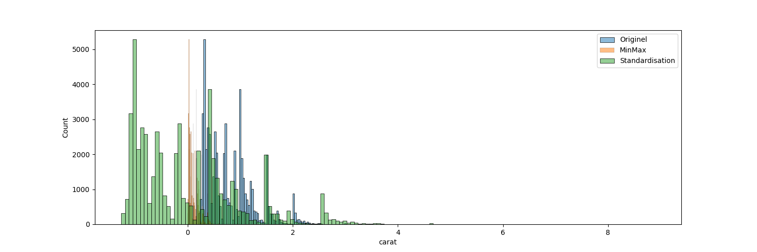
plt.figure(figsize=(15,5))
sns.histplot(data=df_numeric, x='carat', color='tab:blue', alpha=0.5)
sns.histplot(data=df_minmax, x='carat', color='tab:orange', alpha=0.5)
sns.histplot(data=df_standard, x='carat', color='tab:green', alpha=0.5)
Comparatif df_numeric, df_minmax et df_standard (Box plots)
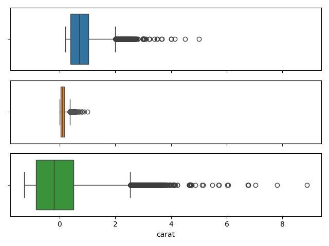
fig,ax = plt.subplots(3, 1, sharex=True)
sns.boxplot(data=df_numeric, x='carat', ax=ax[0], color='tab:blue')
sns.boxplot(data=df_minmax, x='carat', ax=ax[1], color='tab:orange')
sns.boxplot(data=df_standard, x='carat', ax=ax[2], color='tab:green')
plt.tight_layout()
Ni MinMax, ni Standardization => testons les deux
5. Standartisation - Depth
Comparatif df_numeric, df_minmax et df_standard (histogrammes)
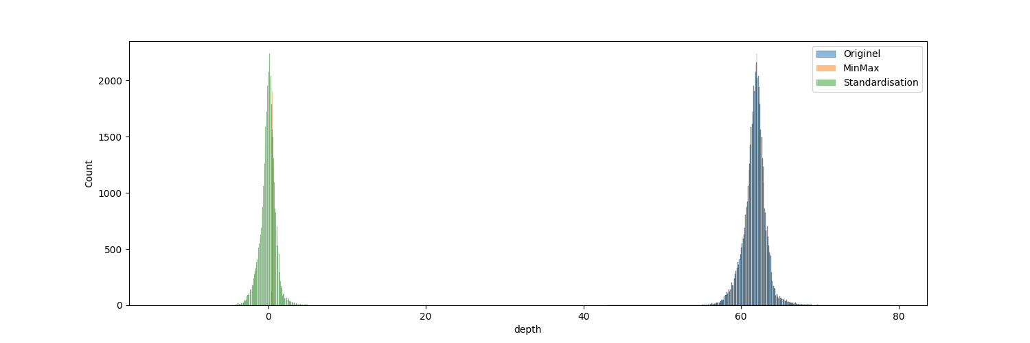
plt.figure(figsize=(15,5))
sns.histplot(data=df_numeric, x='depth', color='tab:blue', alpha=0.5)
sns.histplot(data=df_minmax, x='depth', color='tab:orange', alpha=0.5)
sns.histplot(data=df_standard, x='depth', color='tab:green', alpha=0.5)
Comparatif df_numeric, df_minmax et df_standard (Box plots)
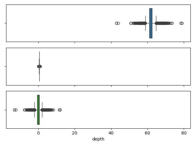
fig,ax = plt.subplots(3, 1, sharex=True)
sns.boxplot(data=df_numeric, x='depth', ax=ax[0], color='tab:blue')
sns.boxplot(data=df_minmax, x='depth', ax=ax[1], color='tab:orange')
sns.boxplot(data=df_standard, x='depth', ax=ax[2], color='tab:green')
plt.tight_layout()
=> Choix de Standardisation
6. MinMax - Price
Comparatif df_minmax et df_standard (histogrammes)
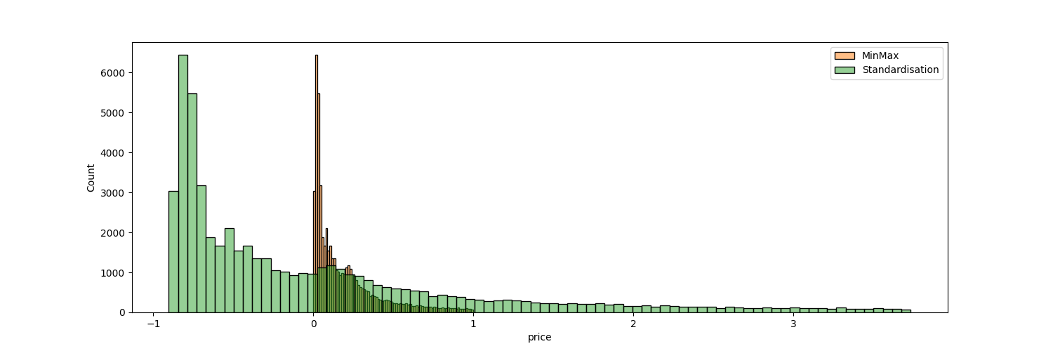
plt.figure(figsize=(15,5))
sns.histplot(data=df_minmax, x='price', color='tab:orange', alpha=0.5)
sns.histplot(data=df_standard, x='price', color='tab:green', alpha=0.5)
Comparatif df_minmax et df_standard (Box plots)
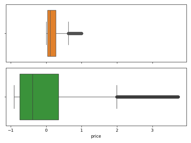
fig,ax = plt.subplots(2, 1, sharex=True)
sns.boxplot(data=df_minmax, x='price', ax=ax[0], color='tab:orange')
sns.boxplot(data=df_standard, x='price', ax=ax[1], color='tab:green')
plt.tight_layout()
=> Choix de MinMax